Andresen Lab Blog

For the most part this week, I’ve been figuring out the optical system and components that we are going to include in the magnetic tweezers setup. It’s been problematic so far, because we’re having difficulty with the parts list from one of Professor Andresen’s friends. Complicating the situation is the fact that they’re in Singapore, so any communication is delayed significantly.

One of the first problems we have is determining how to focus the collimated light coming out of the objective. This light has to be focused in order to be stored on our CCD. We have a choice of either a f=100 or f=180mm lens. However, we’re unsure if (and what would happen) if we include both lenses in the setup at the same time. Secondly, we need to figure out what type of LED we want as our light source. We’re leaning to using Thorlabs as our main supplier for all of our opto-mechanical and optics equipment for ease. So, for the most part of this afternoon, I’ve been chatting with a tech-adviser from Thorlabs for help with selecting the LED and the appropriate opto-mechanical components. Right now we’re leaning towards a red (625nm) LED w/ an output power of 1000mA. To collimate the LED, we’ll be constructing our own collimator out of different Thorlab stuff. We’ll be using an aspherical lens with AR coating in some appropriate housing to collimate the light from the LED. This housing will attach to the LED itself. Of course, the main problem now is making sure that the whole list of everything we need is complete, and get everything ordered.

This morning, I reanalyzed the cobalt- only samples on the ICP, exported the raw data, and added the information to the graphs I made yesterday. The fraction of charge neutralized by cobalt was within the standard deviation from the first run but the individual concentrations of cobalt and phosphorus were significantly lower than yesterday. Although the second run had much lower concentrations, the trendline for both ions traced the same as the first run. This afternoon, I have been catching up on my reading about DNA, nucleosomes, SAXS and studies related to my experiment. 

I recreated the graphs from yesterday of the fraction of charge neutralized by Cobalt and Sodium among others using data from both of the runs. Below are the separate graphs of the charge neutralized by the ions. 

Oggi io ho letto molti documenti per il mio lavoro. In the morning I read up on optics, particularly relating to ccd cameras and camera focusing in general. A problem that we’ve encountered is that, while the focus from the back end of the objective in the setup may be infinity, we still need a way to resolve the picture so that it is in focus for the ccd camera. We need a lens, and a couple of other optics to get the setup to work properly.
I also began to document and review parts lists for other magnetic tweezers setups. I will begin comparing these groups’ parts lists to our own, and figure out which are necessary.
Around 3.30, the motor control board and the motor itself arrived. I began to play with the motor control board by connecting it to my laptop via usb. A green light came on flashing on the board, which is a good sign. After a little hassle, I believe that I have my laptop using the right driver for the control board. Hopefully my pc will now recognize the device.

I analyzed the data collected from my final run last week to determine the quality of the run based on the knowledge I have about how the concentrations of cobalt, sodium and phosphorus change with increasing sodium levels. Using the fact that each of the samples increased in sodium from 0 mM to 80 mM, I created Excel graphs to show the relationships between each of the ions and also how the system competitively behaves. I also determined the relative proportions of cobalt and sodium in solution and created a graph to show their congruence relative to the amount of phosphorus detected. This is shown in the graph below. 

After starting the ICP- OES, I created 5 mL samples including 50 uL of the samples provided that consist of DNA with 1 mM Cobalt2+ and varied amounts of Sodium+ ions dissolved in a solution of KCl and Tris. The samples had sodium amounts from 0 to 80 mM. The samples were run with the calibration of cobalt, sodium and phosphorus that were created previously. I had the chance to modify the method for this run from the method used yesterday. The ICP was then put on standby for Monday and I have several graphs to make on Monday based on the data from today’s run. Hopefully I can put a few of them in on Monday once they are completed.

P.S.

I almost forgot to mention a revelation I had while Prof. Andresen was explaining the physics (mostly thermo) behind what we are attempting to do. For over ten years, studies have been undertaken to determine why, under certain conditions that I don’t remember exactly, DNA will attract another DNA even though they are both negatively charged. The Poisson- Boltzmann equation fits what is observed except for the attraction part. In lab, we are trying to evaluate what is causing this attraction. This leads to my revelation, Prof. Andresen explained this to me today and all I thought about was a scene in Chasing Liberty (a movie about the president’s daughter on an adventure in Europe) and the part where the president’s daughter was a “Chickie buffer (that) negates the potential for man-touching-man discomfort” so that the two guys in the movie could hug with her between them. So this summer, I am trying to find the chickie buffer!

Today I delved into some LabVIEW code that we will be using for our magnetic tweezers setup. We identified the sub VIs pertaining to motor control and basically figured out how they work. We also identified possibilities for future motor control.

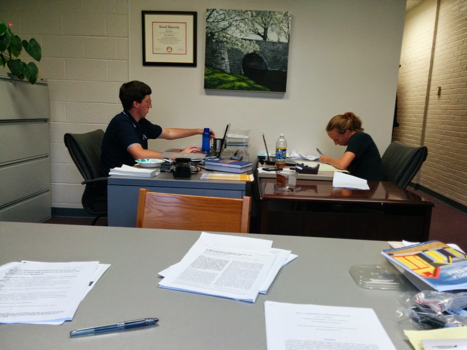
Abby and Steve hard at work in our newly created student office!

The summer has begun with two great new students (and the same old professor). We have a couple of great projects going on this summer from building a new instrument from the ground up to continuing our quest to understand the physics behind DNA packing! (In fact they have gotten some posts in ahead of me below.)

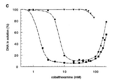
From Pelta et al., Journal of Biological Chemistry, 1996

Abby Bull will be working on the DNA packing part of things. In particular she will be trying to understand the graph at the right. What this is showing is that as cobalthexammine (the chemical is not important, just know that it is a +3 ion) DNA clumps together (aggregates) and falls out of solution. This is surprising because relatively small amounts (~5mM from this graph) of CoHex can do this while there is no amount of +1 or +2 ions that you can add to do the same thing! It is something particular to +3 ions. (Those of you who are observant may also notice that something equally strange happens when you keep adding CoHex.)
Abby will be looking at “pellets” of DNA that are have been put in the state at the bottom of the “valley” in this graph. Ones that have condensed/aggregated/clumped together. Our collaborators at George Washington University have made these samples and then redissolved them in a different solution (in this case a highly concentrated KCl solution). They have made many of these samples, systematically changing the ratio of +3 ion (CoHex) to +1 ion (NaCl). Abby will be measuring the amount of +3 ion and +1 ion that was actually bound to the DNA when it was in its “clumpy” state. Using this, we hope to extract the physics, in particular the forces between DNA, that lead to this state. This is a follow-up on some work done previously by John Giannini in our lab that looked at the amount of +3 ions and +2 ions that were bound in the same state.

Image courtesy of Wikipedia

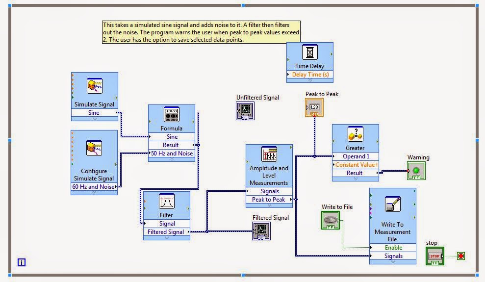
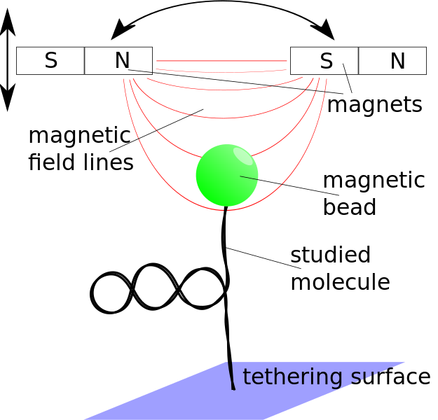
Steve Kenyon will be working on building a magnetic tweezers setup from scratch. What are magnetic
tweezers you may ask? In magnetic tweezers, one uses small (but strong!) permanent magnets (think refrigerator magnets on steroids) to pull on small magnetic beads that are attached to the object of interest. In our case we often are pulling on DNA or DNA with other proteins interacting with it. By carefully calibrating the machine one can measure exactly how long the molecule of interest is when you pull it with a certain force. By measuring how hard it is to pull the molecule straight, we learn something about the structure of that molecule before we started pulling on it. (Just like you can tell how tangled a telephone cord is by how hard it is to pull the cord straight.) (I know those of you who are younger out there may be wondering what a “telephone cord” is. Pleas ask your parents.)
This is a pretty involved project that will involve writing a lot of computer code in a funny computer language called Labview and doing a lot of interfacing of physical instruments, motors, and cameras with the computer and the program that is running it. All-in-all a great introduction into machine design!

So, I hope you will all enjoy our journey this summer with us and hopefully will be cheering us on as we race to get all of this done before classes begin!

Day 1

Fig 1: This is an example of the decision maker program. The top shows the front panel of LabVIEW, which displays the output of the code. The bottom is the block diagram, the code itself. For an input temperature and current machine speed, the code determines if the machine is running too hot. If it is not running too hot, it allows the machine to speed up.

Fig 2: This program creates a sine signal and then adds noise to it. The unfiltered sine signal is displayed for the user graphically in the front panel. The signal is then filtered and displayed for the user. The code displays a warning signal to the user for peak to peak measurements of the filtered signal that are above a threshold. The user also has the option to press a button on the front panel that allows them to save certain data points to a text file.

Day 3

I started up the ICP with help from Prof. Andresen, including putting new tubing on the Peristaltic pump. I ran a calibration set for 50mL solutions comprising of 0-500ppb of Na, Co, and P for a total of six calibrations. These were also used as the samples. In the afternoon, I read through the software manual and then Prof. Andresen and I reprocessed the samples from the morning and reviewed the data.