ITC (I Try Coding)

Hi everyone! My name is Danielle and I’m working with Dr. Andresen on modeling DNA binding and condensation. In the past few years, I’ve been working with the isothermal titration calorimeter, or ITC, which I wrote about here and here. For the first few weeks of this summer my goal has been to collect more ITC data and to write a python script to fit the data. Fortunately, these pursuits have been going very well!

Figure 1
Integrated ITC data showing the binding and condensation of DNA. [1]

If you read my previous posts, then you’ll notice a major difference with the above picture. That difference is the presence of a second peak, representing the condensation phase of the binding process. What this means is that the DNA first binds to the ligand, (the injected solution—in this case, cobalt hexamine) then when the concentration of ligand increases to a certain point, the DNA condenses into a smaller, more energetically favorable shape.

While this is certainly very interesting, it provides a significant challenge to model mathematically. Fortunately a model was created for this very situation by Kim et al. [1] The equations, shown below, are very complicated so I won’t go into how they work too much here.

Equation describing the heat released during titration. This allows us to fit the parameters N, K, and ΔH. [1]
This function tells us the difference in heat between injections. It is normalized then normalized before being fit. We call the normalized function NDH. [1]

On top of these long equations, the fitting process itself is very complicated. We actually have to add up multiple NDH functions before we can fit the parameters. The first of these, NDH1, gives us the parameters N1, K1,and ΔH1 and fits the first binding stage. The second function, NDH2, describes the second binding stage and is composed of multiple other functions. This gives us the parameters N2 = N2‘ – N3, K2,and ΔH2. Finally, we add up NDH1 and NDH2 and fit the parameters with that function. In the end, this means we’re fitting 7 variables simultaneously!

This has meant a lot of programming in the past few weeks. The first step was to recreate a graph from Kim et al. to make sure that the model function actually worked. It took a while, but I was eventually able to get it to work.

Graph showing the components of a fit. [1]

My recreation of the same graph. The slight differences are probably because I generated a slightly simpler set of sample data.

Once I got this part to work, things were relatively straightforward. One week, two data fitting packages, and many, many mistakes later, I was able to get 100 lines of code that can (theoretically) fit any set of double-peaked ITC data. My next steps are going to be doing some version control with Git, adding more features to my fitting function, and cleaning up my code. Hopefully, I’ll have a fully functional python script on GitHub by the end of the summer, if not sooner!

Sources

  1. Kim et al. “Development of a Fitting Model Suitable for the Isothermal Titration Calorimetric Curve of DNA with Cationic Ligands.” The Journal of Physical Chemistry. 110, no. 22 (2006): 10919–25. https://doi.org/10.1021/jp057554e.

Ion Competitions and Programming Headaches

Hey! I’m Matt, one of the researchers working with Dr. Andresen this summer. My project is a continuation of a published work Dr. Andresen collaborated on back in 2013 (link). Allow me to give you some background before I explain exactly what it is I’m doing. The electrostatics of nucleic acids are fundamental to both nucleic acid structure and function. The physical origin of DNA condensation -a process essential for gene regulation- remains unsettled. It is the goal of our research to further our understanding of both these aspects/processes by observing what happens to DNA condensation when the solution containing the DNA has different amounts of differently charged ions. The research Dr. Andresen worked on in 2013 explored what happens when the amount of +2 and +3 ions varies in the solution, my research is interested in +1 and +3 ions. Basically, we look at how many of each ion bind to the DNA as their concentrations vary. My job, more specifically, is to simulate the DNA ion-competition according to how the Nonlinear Poisson-Boltzmann (NLPB) equations say it should work. Practically, this means arranging the DNA strands into predetermined shapes (in our case a hexagon) to try and mimic a small strand of DNA in vitro. Hopefully, our research will provide more insight into, not only into DNA condensation, but also biomolecular electrostatics in general.

As for my work these last few weeks, it’s mostly been trying to learn (and then unlearn) a few python packages for working with .pdb files. .pdb files are files with specific formatting that stores information about the DNA like its positional data, total charge, connections between nucleic acids, etc. This started off pretty well with me making rapid progress in terms of positioning the DNA strands where they needed to be (see below), but sadly, as I learned this Thursday, the packages I was using to do this unfortunately break the .pdb files when they edit them. Not break them completely, mind you, but just enough where the accuracy of the simulation takes a serious hit and thus I had to abandon them. This left me with only one option: write my own. Fortunately, I don’t need much of the functionality of those packages, I really just need the ability to modify the positions of the strands. I imagine I’ll have this done sometime early next week as the only snag left is that .pdb files require a very specific format that is whitespace dependent and I’m having trouble getting everything to literally lineup as it should.

DNA strands arranged in a Hexagon. VMD is the visualization software


After I work out the kinks, the next step will be to run my .pdb file through https://server.poissonboltzmann.org, a free Poisson-Boltzmann equation solver. This allows me to outsource the processing of the data to a webserver so my poor laptop doesn’t overheat and die trying to do all that math. Once I get the data back and in a state that I deem acceptable, I’ll be able to start doing some actual analysis, but at this point that’s getting ahead of myself.

Nanoparticle Lab Week 1 & 2 Report

Hello! My name is Thomas Gilman. I am working on the gold nanoparticle coating lab under Dr. Andresen and Dr. Thompson’s collaborative project. In this project we are aiming to wrap DNA around gold nanoparticles and be able to characterize them to see the treatment potential they have on diseases in the human body, such as cancer. In wrapping DNA, the nanoparticles must first be wrapped in a positive charged polymer, PAH (polycyclic aromatic hydrocarbon). Once this has successfully been completed, the DNA is then coated onto these nanoparticles with PAH already wrapped onto the gold nanoparticles. These particles are characterized through UV-Visibility spectra, which measures the absorbance of the sample; DLS (Dynamic Light Scattering), which measures the size of the particles in the sample; and Zeta, which measures the Zeta potential of the sample. Through characterization, we will be able to see the success of the coating and determine the possible further uses of such particles.

In the first week, we completed trial runs of the first step of the coating process which was the initial coating of PAH on the gold nanoparticles. Our initial runs were conducted including a 10:2:1 ratio of the nanoparticles, PAH, and NaCl, respectively. With these samples, we allowed for a coating time of 30 minutes. After the 30 minutes concluded, the samples were run through the centrifuge in order to create a pellet of the coated particles. The samples were then run through a cleaning process to remove excess non-coated particles and solution components, and then the remaining pellet was resuspended in water. These resuspended samples were then run through the characterization tests described before. Our data, shows that there is slight aggregation with the 30 minute coating sample having the 10:2:1 ratio (Figure 1) seen in the separation of the data line and the normalized line between 575 and 700 nm. With this, I then conducted the same test again, as well as comparable 24 hour coating time samples (Figure 2). After concluding these tests then, it was found that the longer the coating time, the less the aggregation present among the nanoparticles. This lesser aggregation can be seen in the normalization graphs presented as well, with the curves being more matched together for the 24 hour sample, compared to the 30 minute sample. 

With this data, and the overall success of the initial coating with PAH, the next steps are to look into coating these wrapped nanoparticles once more, now with DNA. In order to do so, the DNA must be sheared and prepared first to be added to the existing solution in order for a more successful wrapping. For week two, this was our focus, and being able to do the first test coating on a smaller sample on Thursday, and letting it coat for 16 hours overnight into Friday. In the meantime I made larger sample sizes to be ready, in the best case scenario where the DNA successfully wrapped around the nanoparticles. This will be measured through the same tests as mentioned before, where the success will be measured by a higher absorbance (meaning a high concentration), a larger size (meaning there is the extra layer onto the particles), and a negative Zeta potential (meaning that the DNA successfully wrapped and charged the charge of the particle). Stay tuned to know if these tests were successful next week!

Figure 1: UV-Vis Graph for sample TG 5.28.21 30 min 200 µL Citrate Au Nanoparticles with significant aggregation present between 575 and 700 nm present

Figure 2: UV-Vis Graph for sample TG 5.27.21 24 hour 200 µL Citrate Au Nanoparticles with minimal aggregation present in the region of comparison from the 30 min coating sample

The Andresen Lab is Back!!!

We got a bit of a slow start to the blog, but we’ve been back now for a couple of weeks and are ready to continue teaching everyone about the great science that is going on in our lab. We’ve got a strong crew this year led by veteran Dani Wallace and with two strong newcomers Matt Day and Thomas Gilman. I can’t wait to see all of the great work everyone does! (And I’m sure you can’t either!)

If you really can’t get enough of us, we have an RSS feed and you can check out our (static) lab website. I’m also hoping to get a twitter feed figured out soon, so stay tuned!

Working so hard on the first day!!! 🙂 Hopefully they are still smiling at the end of 8 weeks!

Week 6 & 7 – DNA Wrapping & Starting Over

During the beginning of week 6 and 7, I continued DNA wrapping. I tried using different concentrations of each the DNA and AuNPs, however, nothing worked well. I could not replicate my very first try, which, although was not useable due to excessive aggregation, still was indicative of wrapping due to the surface charge flip from positive to negative. After trying to wrap with this sample multiple times, I concluded that these particles were simply not useable for wrapping even though the measurements were not bad. To confirm my suspicions, I still had a little bit of the pellet I used for my first attempt at wrapping, so I tried it again with that. As expected, the surface charge flipped, indicative of some wrapping. So I threw my new samples out.

Attempting to start again with wrapping, I noticed I had old citrate particles that were very good lying around. I didn’t want to waste good particles, so I tried with these. It ended up being a waste of time. I coated a bunch of them with polymer, which worked out very well, and cleaned them and pelleted them. These looked much better than the other samples that I had been using.

These are old particles from the beginning of research that looked very promising under the UV-Vis. As you can see, every step is not aggregated at all and is only widening a little bit. I was hopeful that these might work.

After calculating the concentration using the method I used before, I diluted the pellet 10x in order to keep them from being too concentrated. The pellet ended up being at least 2x more concentrated than the previous pellets, so I didn’t have to waste as much in order to make the same amount of solution.

After wrapping, zeta potential showed that the surface charge was still positive. However, it was only slightly positive at around 12mV. This is indicative of slight wrapping, but the majority of particles were still not being wrapped. I concluded that this was most likely due to the sample not being cleaned enough, and there was simply too much PAH floating around that the DNA could stick to instead of the particles. So I tried to clean my samples again to see if that would help. Unfortunately, this completely destroyed them in the process. The data was extremely weird, the sample looked extremely polydisperse and they had probably the most horrible looking absorption spectrum I’ve ever seen. However, the surface charge was 0mV. From this, I decided no more. I was going to figure out how to clean the particles and remove excess polymer without aggregating them. So I looked through a bunch of different papers.

Moving on to week 7, I had looked through a lot of different papers that coated AuNPs with all different kinds of polymers. A lot of the papers said that they centrifuged the particles at high speeds of 9000-12000rpm for a short amount of time (5 – 15min). I was surprised at this but decided to give it a try. I ended up going with the same speed and time that the people in the chem department used in order to coat with polymer, 9000 rpm for 15 minutes.

I also noticed something in the papers. Almost all of them had some form of saying, “in order to keep samples as good as possible, we always used freshly made particles for our experiments”. I realized that maybe freshly made particles are just better to use than old ones, for some odd reason. It’s probably because it’s super hard to make perfectly stable particles, so they’re always going to worsen a little bit over time. So I made new particles, batch 4, and went through all the steps. They looked very promising every step of the way.

Next week I’ll start making DNA-AuNPs using my new particles.

Weeks 4 & 5 – Nanoparticle Pellet Preparation & DNA Wrapping

During the beginning of these weeks, I focused on perfecting the polymer coating procedure from before. I got a few good attempts, in which the data looks decent enough to move on to DNA wrapping, but overall, there is no deciding procedure that works the best. This is somewhat disappointing; when I need to make new PAH-Cit AuNPs in the future, I have to either get lucky or find a way that does work most of the time. For now, however, I am going to use the ones that are decent enough to move forward. These are all from the same batch but are separated into 15mL conical tubes in order to make the centrifugation go smoothly. Their absorption graphs look decent, with only a small shoulder which indicates some aggregation of particles. This isn’t too big of an issue, though, so they are cleared to wrap with DNA.

In order to get the particles ready for DNA wrapping, I needed to make the concentration higher. The concentrations were extremely low which would not work very well. To do this, I centrifuged them at 4000rpm for 45 minutes, removed the supernatant on top, combined the pellets and recentrifuged the supernatant until no pellet emerged. This would eventually give me a concentrated sample of NPs. 


I also needed to prep the DNA for wrapping. To do this, I made a sample of DNA dissolved in TRIS buffer that has a steady PH. Once dissolved, I sheared the sample with a probe sonicator. This is a technique that essentially shortens the DNA to a specific length that allows for wrapping. The machine makes a really loud noise, so I had to wear ear protection. After this, I realized I used the wrong concentration of TRIS buffer before, so I had to dilute it in ultrapure water (deionized to ensure the DNA’s charge was not messed with) and a certain concentration of NaCl, which is needed later in the process to ensure the DNA and polymer are all surrounded with charges, but we decided to add it in then to save time. I also measured the absorption spectrum of both the sheared and unsheared DNA samples, in order to obtain their concentrations. This didn’t turn out well.

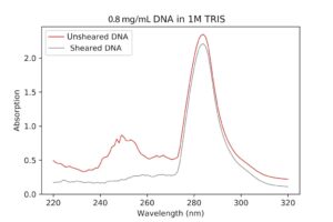
Sheared DNA VS Unsheared DNA UV-Vis spectroscopy. The peak should be at 260nm, but it’s much higher. I’m not really sure why this is, although it might have to do with the machine not being calibrated correctly or my TRIS concentration being too high. 

Once the sheared DNA had been buffer exchanged, I ran another UV-Vis characterization to see if they were any better. I then realized I had been using a plastic cuvette to measure the spectrum, which, if you know anything about physics, is impenetrable by UV rays. Since the wavelength parameters are set to numbers in the ultraviolet range, I wasn’t actually getting real data. So, I re-ran the measurement with a quartz one, and they turned out good, with peaks of about 260nm (expected).
The absorption value at the peak, 0.13587, enabled me to calculate the concentration of DNA in the solution, which turned out to be around 0.68 mg/mL. For wrapping, I need to dilute this by about 10x.

Meanwhile, I finished pelleting my particles and needed to calculate their concentration with the UV-Vis as well in order to start wrapping.

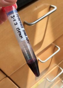
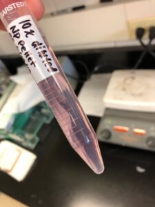
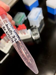
Extremely concentrated gold nanoparticles. This is only about 2mL, as each time the pellets are combined it only adds a few μL of particles. These were already cleaned with the centrifuge process before pelleting.

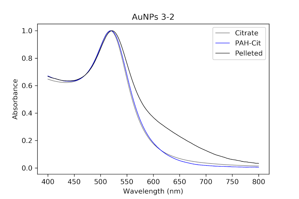
When I ran the UV-Vis I had to dilute the pellet 100x. The particles looked decent. Some mild aggregation and thickening of the peak had occurred, but I deemed this not significant enough to not continue wrapping. In python, I programmed the files from the machine in order to set up a graph, as usual. However, this time, in order to clean the samples, I needed to separate them into smaller tubes, 8 to be exact. There were 8 samples that looked extremely similar to one another and were going to be recombined anyway. To get the picture that you see below, I attempted to take the mean of the absorption values of all 8 samples at each wavelength, normalize them, and plot them again as a new line. This took me two hours, but it was worth it, as now the graph is much cleaner looking and easier to understand.

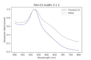
The original PAH-Cit AuNPs cleaned twice with a centrifuge versus the pellet solution (a dilute version), normalized. As you can see, the pellet has a thicker peak and a slightly bigger shoulder.

With this data, I used the Wolfgang Haiss protocol from another academic paper in order to determine the concentration of the particles. The procedure is as follows: take the absorption value at the highest peak, divide it by the absorption at 450nm, use the table to determine the diameter, and then use another table to determine the molar decadic extinction coefficient, which can then be used in the equation c = A450/ε450 in order to determine the concentration in moles. All of the calculations have been done in the paper, so I simply had to follow the protocol. When I did this, I finally got a concentration of 39nM for my pellet. I then diluted it by 10 in order to not overwhelm the DNA.


The first ingredient for the final mixture, diluted pellet from my PAH AuNPs.
                                                

I diluted the DNA 10x simply by combining 1mL with the particles instead of diluting it with water and then adding 10mL, which is essential because I don’t want the water to contaminate the concentrations of NaCl and TRIS that the DNA is combined with. This gives me a final concentration of 0.068mg/mL DNA.

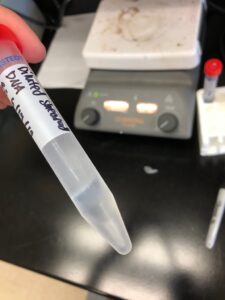
The second ingredient for the final mixture, diluted sheared DNA.

This is my first attempt at creating DNA-PAH-Cit coated AuNPs. I shook it vigorously in order to make the DNA wrap around the particles, which Dr. Andresen said might work because we really have no idea what we’re doing and we have to try something. I then left it overnight.

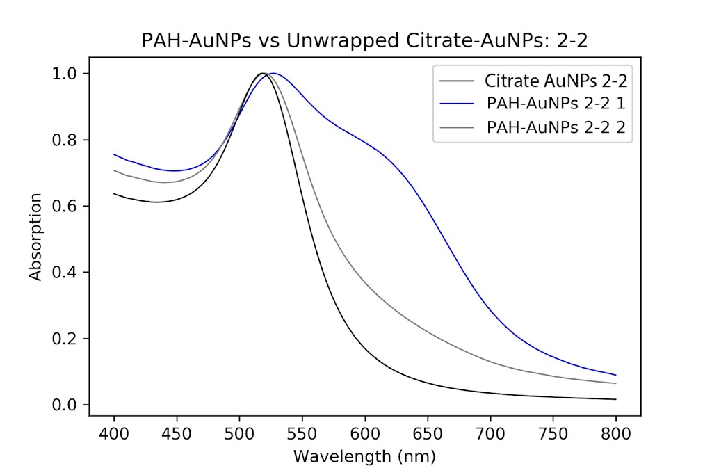
The next morning, they were a little purple in color. I ran UV-Vis measurements as well as DLS and Zeta potential. The absorption spectrum looked worse than the pellet, which I guess is to be expected, but since the pellet was already kind of aggregated, it made it worse.

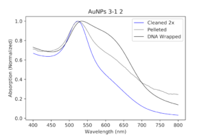
My DNA wrapped particles compared to the original cleaned and pelleted polymer particles. The black line, indicative of the DNA wrapping, is aggregated. Ugh.
                       

I still wasn’t completely sure if this was terrible or not, so I began to clean the wrapped particles 2x in the centrifuge and run the tests again to see if they were better. After cleaning, I noticed that the tube had a clump of aggregated particles at the bottom and I immediately knew they weren’t going to be useable, but I still ran them through the UV-Vis, confirming my doubts. So much for the first attempt.

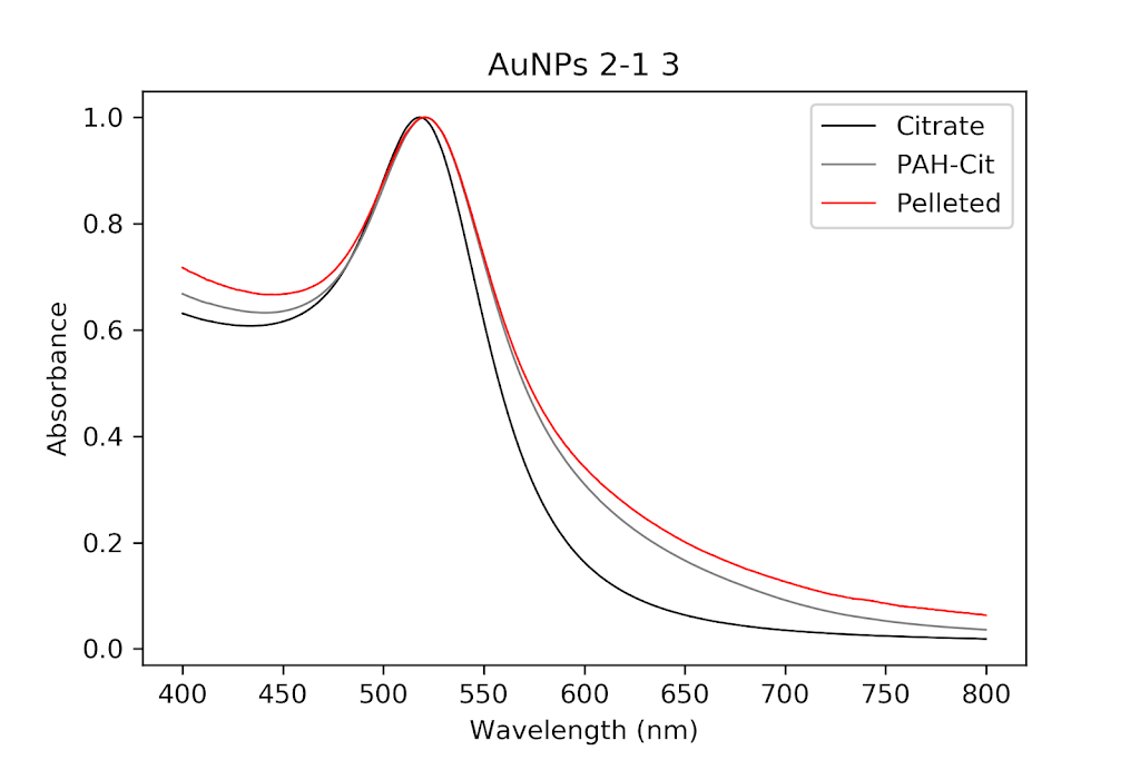
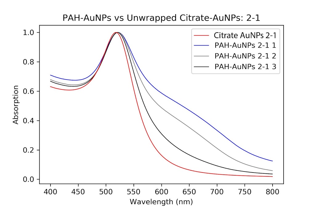
I decided to redo wrapping, but with a different set of particles. Luckily, I had other even better PAH ones that I had been pelleting along with the others and eventually worked my way up to 1mL of pellet. I then checked their absorption spectrum to ensure these were still as good as they were before. These particles were so much better it was insane. There was almost no shouldering even on the pellet solution, as opposed to my first try. 

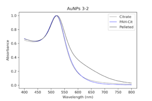
Pelleted particles compared to original citrate and PAH-coated particles. As indicated by the black line, there is almost no aggregation and only slight broadening of the peak that has occurred. This has potential.

I knew I had to save as much of this pellet as possible and not waste it with possible aggregation with DNA each attempt. I decided to dilute the pellet 50x instead of 10x in order to save the particles for as many tries as possible. I made 3 samples of the diluted pellet because the pellet has a greater chance of aggregating on its own if let sit out, simply because the particles are more concentrated and closer together. I only used 200uL for each dilution, which is great. I calculated the concentration using the method from before, and then I mixed the two ingredients together, 1mL sheared DNA from before and 9mL of the diluted pellet, in order to make 10mL of the DNA wrapped particles. Instead of shaking it vigorously this time, I decided to invert the tube a few times and let it sit a while instead. I noticed that I did the same thing when coating with PAH, and even when I made the original citrate particles. I didn’t disturb them at all, I just mixed them a little and then let them sit. I was hopeful that this would not cause aggregation but would still allow for the DNA to wrap around the particles.

My DNA-PAH-Cit AuNPs attempt 2. As you can see, they are a nice pink color, as opposed to the purplish color that arose from the previous try. These should be better.

I then let them sit for a few hours and ran UV-Vis and DLS/Zeta on them. They seemed a little weird – the UV-Vis looked somehow unchanged from the dilute pellet, which was strange because I was expecting at least a little aggregation. The zeta potential was also weird because the surface charge was about 40mV. I was expecting this number to be negative since DNA is negatively charged, so I guess wrapping didn’t occur. The pellet’s charge was about 55mV, so I guess it did reduce it a little, but not nearly enough. It should be around -30mV. I deduced two things from this. Either the wrapping didn’t occur because I didn’t shake it enough (maybe the particles are stubborn), or I didn’t add a high enough concentration of DNA, so not enough stuck to the particles. I’m not sure what concentration to do next, or if I should stick with the original and try to shake it a little more. I’ll do that next week.

Finally, I started pelleting my other particles that were good, even though they are only 10mL each. Next week, I’ll finish pelleting these for later on, as well as make a new batch of DNA wrapped particles probably using a different concentration. I’m just happy that I was able to progress to the final step of preparation in my research. After I get these and they look good, I can begin experimentation. Hopefully, they work out!

Update on preparation of nucleosomes

I am about 4 weeks into research (half way done with my research here on campus for the summer) and so close to having mononucleosomes. Since the last time I posted, we have made progress on preparing nucleosomes. The past couple of weeks have consisted of digestion processes with the DNA and running gels to try to figure out if we had nucleosomes in our samples.

Figure 1: Column Trace of NCP (nucleosome core particle) prep samples


Last week, Dr. Andresen ran a column with the samples we have of DNA. Figure 1 shows the results of the column which helps us determine what each sample has. Each green number indicates a sample number. Thus, we can conclude that samples 1-9 have di and trinucleosomes, where as samples 10-14 have mononucleosomes and the other samples have left over DNA. Therefore, from the column trace we were able to determine that we have mononucleosomes and which samples they are in.  
Figure 2: NCP prep gel run with DNA ladder

Earlier this week I prepared samples to run through 1.2% Agarose gel. As shown in figure 2, we ran 18 samples (4-21) with two DNA ladders on each end. We ran the DNA ladders with the samples because the DNA ladders indicate the length of the nucleosomes. As you can see in figure 2, the red lines indicate how many base pairs there are in the samples, thus distinguishing whether there are  mono/di or tri nucleosomes in the samples. As we had assumed, samples 10-14 most likely have mononucleosomes. We were able to conclude this because one nucleosome has ~147 base pairs and the gel we ran shows us that those samples are closest to having the length of a mononucleosome. Even so, Dr. Andresen is going to discuss our results with Dr. Beuttner, in the chemistry department, in order to confirm what samples we should use to proceed. Even so, I believe that we will continue to purify the samples to try to get as many mononucleosomes as we can. 

Also, now that we are closer to having nucleosomes, I am working on learning how to use the Inductively coupled plasma-optical emission spectrometry machine in the lab. The ICP-OES machine is used to determine the concentration of elements in samples. Thus, I have been preparing samples to run test trials and familiarize myself with the machine as I will be using it to run actual experiments with the nucleosomes.

Week 2 – Polymer Failure

With last week’s nanoparticles, Dr. Andresen and I decided to focus on citrate for now and start coating citrate AuNPs with a polymer. The reason we do this is that citrate is negatively charged, which is the same as DNA. Coating the particles with a positively charged polymer such as polyallylamine hydrochloride creates an opposite charge for the DNA to cling to when we begin to wrap it. I started this week by attempting to coat the particles with the polymer. To do this, I made a sample of polymer dissolved in a solution of 10mM NaCl so that the polymer’s concentration was 10 mg/mL. I then made a ratio of 10:2:1 of citrate AuNPs, stock polymer solution, and 10mM NaCl. I didn’t want to waste many particles, so I only did 10mL to 2mL to 1mL each batch. Unfortunately, during this process, I contaminated one of my original citrate batches and the whole thing turned black, rendering them useless. I still had one good batch, but I also picked up a new batch that Dr. Thompson made and used those two to make polymer coatings. Unfortunately, I failed both of my batches, with both of my samples in each batch looking horrible on the UV-Vis spectrum. What we are looking for is a slight redshift (shifted right towards the red side of the spectrum) that shows that the polymer has attached, as well as the same peak shape as the uncoated particles. The particles will obviously get a little bigger when coated with something, so if there’s no redshift, the particles haven’t been coated. When I finally got to the third attempt, the data looked decent. I was starting to see progress, but they still weren’t great particles. At this point, I decided to try a new method from a scientific paper that someone did that was related to my topic. After trying this and collecting the results, it turns out that the new method is even worse than my original one, so I’m sticking to the old fashioned way. I also was able to make the absorption graphs in python after some tinkering with the code, and I normalized the data (made the maximum value in the data set 1 and scaled everything accordingly) in order to make the redshift clearer.

PAH-Cit AuNPs compared to their original unwrapped citrate AuNPs sample 2-1 (the red line). The blue line shows complete aggregation and is not a good set of data. As time went on, however, the method became muscle memory and the blue to grey to black lines show this progression. There is a slight redshift that occurs, which indicates growth.
PAH-Cit AuNPs in the second batch compared to the original unwrapped citrate AuNPs sample 2-2 (the black line). The same pattern is clear here as well. 
After a decently successful UV-Vis characterization, I went on to review the size DLS and zeta potential measurements. The size DLS was terrible overall, with all of my bad particles showing double peaks which indicate polydispersity (not all the particles are the same size). My good particles showed double peaks as well, however, I wasn’t worried due to intensity (the y-axis on the graphs) being related to size as a factor of 10^6. This means that even though the peaks look relatively the same, the peak that shows particles with a bigger size is scaled up enormously. 
PAH-Cit AuNPs sample 2-1 3 size DLS results. The graph shows double peaking at 34 nm and 122 nm, however, almost all of the particles are around 34 nm, which is to be expected since the polymer layer only adds a few nanometers to the particle’s diameter.
The zeta potential results for all of the particles were good, anywhere from 30 to 40 mV. Since they are positively charged now, it means the coating went well. However, this does not give any indication of how monodisperse the particles are, so even the bad particles had a good charge. Next week, I am finally going to start to coat my particles with DNA. I don’t have very many particles left after all my tests, so I’ll make some new ones to wrap. Hopefully it all goes well.

Week 2: Data Time!

Learning to use the ITC over the past week and a half has been a long process. At the beginning of the week, I got some pretty terrible results. Here’s a small selection from the many failures I encountered.

Over time though, the results slowly got better. The goal is to have a smooth “hill” formed by the injection peaks which returns to a flat baseline about halfway to two-thirds of the way through the experiment. Here’s a few my good data sets, which I was able to collect some good numbers from.

I was able to gather four pieces of data from this. The first is the binding energy, Kd. This is a measure of how strong the bond between two chemicals is. The next important number is the stoichiometry of the reaction, n. This represents the ratio of chemicals needed for the reaction to take place. Third, we have the change in enthalpy, delta H. This value is related to both the change in temperature and pressure/volume during the reaction. The last constant is the change in entropy, delta S. This is more or less a measure of the increase in disorder caused by the reaction.

The following graphs were obtained by plotting the area under each injection peak versus its peak number, and then fitting a curve to the data points. This gave us some very consistent results which were also pretty accurate. This is a good sign for future tests!

First week into the process of preparing nucleosomes

On Monday, Dr. Andresen and I began the process of preparing nucleosomes. We began with 50mL of chicken blood which if you’re wondering the reason behind why we use chicken blood, it’s because unlike our red blood cells, chicken red blood cells have nuclei that contain nucleosomes.

First off, Dr. Andresen and I began the process of preparing nuclei. We made 500mL of KTM buffer, which contains Tris HCL, KCl, MgCl2 and PMSF, and combined 50mL of it with the 50mL of chicken blood. Then we spinned that using a Centrifuge machine. The Centrifuge machine separates the heavier stuff (the pellet) from the lighter stuff (the supernatant) by increasing the gravitational force.Therefore, for the first couple of spins it helped us separate the red blood cells (the pellet) from the extra stuff that the blood contains such as plasma (the supernatant). Then, we resuspended the cells in KTM buffer and Triton X. The Triton X is like a “soap” which helps “break” the cells in order to release the nuclei inside of them. We had to do this because we want what’s inside of nuclei, the nucleosomes.

Tuesday, we had a discussion about unproductive and productive stupidity in STEM. Right after the discussion, I actually made a mistake and added too much of one solution to a batch of KTM buffer that I needed to use in order to finalize the preparation of the nuclei. Dr. Andresen realized that I did this once he noticed how hard the pellet (which contained the nuclei) was since it wouldn’t dissolve in the KTM buffer. Therefore, I had to start all over. I was frustrated at the fact that I had ruined a day of work but it actually helped me get over the fear that I had of messing up. It began my journey of understanding that research is a process of trial and error and that my mistakes will only help me learn and grow.

For the remainder of the week, Dr. Andresen and I went from having nuclei to having chromatin. When we had the nuclei, we measured how much DNA we had using the UV/VIS machine, which told us the concentration of DNA we had. We had about 125mg of DNA. Then, we resuspended the nuclei with CaCl2 + ML buffer, which contains Tris HCl, NaCl, MgCl2 and PMSF, and heated it at 37 degrees Celsius for 35 minutes. We heated this because throughout the process, the solution actually eats at the membrane of the nuclei which then breaks the nuclei and releases the DNA and everything else in the nuclei. Then, we continued by doing different steps in order to get the chromatin which consisted of making other solutions, spinning it, and letting it sit overnight with different solutions in order to get rid of the extra stuff such as ions and molecules surrounding the DNA.

As of today, Friday, we have chromatin, which consists of DNA linking nucleosomes together. Ultimately, what we’re trying to do is get the nucleosomes, which is an octamer wrapped around twice by DNA, so we’ll have to cut the DNA linking the nucleosomes in order to get the nucleosomes alone. Also, today we measured how much DNA we have, which is approximately how much chromatin we have. We have 37mg of DNA which is about 30% of how much we had last time we had checked. We are hoping to at least have half of this amount by the end. However, during our group meeting today I found out that the next step is where things have gone wrong in previous years. Even so, I am hoping to have some nucleosomes next week.