Ithaca Waterfalls!

After four days of running samples for 16 hours each day, we finished our BioSAXS experiments. But before we left, we went to see several of the amazing waterfalls in Ithaca. 

Path leading up to the largest falls. Unfortunately the path was closed further up because of construction, so we had to circle back and follow another path to the waterfalls. 
WATERFALL!!
Prof. Andresen attempting to take a panoramic view of the falls. 


Week Three: TUESDAY

I started the day off by figuring out once again what the initial motor position would be if I connected everything up to the computer and ran the motor control code. Once again, I found that it was initialized to -16,777,216. This number must have some meaning, but I am not sure what.

Following this, I attempted to figure out how to do a little programming challenge to see if we could make the motors do what we want them to in the long run, or figure out if the existing code we have can accomplish this. The task is as follows:
1) Tell the motor to rotate 3.5 turns and stop.
2) Move back 1.2 turns and stop.
3) Report the position as 2.3
4) Save this position so that when the program is closed and reopened it still recognizes that the motor is at 2.3, ceteris paribus.

As it turns out, this is a bit more difficult than it would seem. The reason for new positions in the motor becoming zero each time the control board is unplugged as opposed to the program being closed and reopened is because the motor position is stored in the control board’s memory, not the program’s.

So how difficult is it to create a vi to do what was described above? Not very, but you need to have the right tools. Tasks 1) through 3) can easily be accomplished with the base code that I’ve been working with, but the unit “turns” would have to be figured out empirically. This is not optimal, so I set out to figure out what the units were, and more importantly, how this motor code works in the scheme of the whole program.

It turns out that the units, speed, and voltage of the motors can all be calibrated in a nice little calib.ini file. This file is then called by a CalibConstants.vi which appears everywhere in the overall tweezers.vi code structure. This CalibConstants.vi should be able to figure out the units and normalize instructions from turns to what the base code I was using earlier uses for units.

CalibConstants.vi is unfortunately not run-able because there are two important files missing: Reset Position.flx and Read Position.flx. The observant reader would note that these file endings are different for every other LabVIEW file that I’ve discussed so far. That’s because, (after doing a little bit of research) these files are related to the NI-Motion set of *stuff*. .flx are Flex Motion files, used by the NI-Motion driver. These .flx files appear several times throughout the tweezers.vi and are most of the missing files in all of the code.

With the inclusion of these two .flx files, CalibConstants.vi should be run-able, and by extension, simplemove.vi, which is the overhead code for the base motor code I’ve been using, which should mean that the programming task I outlined above is entirely executable by the existing code we have. Also, since much of the tweezers.vi code has CalibConstants.vi throughout it, more of that code will be run-able too. This is exciting since our camera and other optics equipment just arrived today.

So what’s the bottom line? Either we rewrite the code or get this NI-Motion driver which should contain the .flx libraries. I did manage to comment out sections of the CalibConstants.vi and SimpleMove.vi that referred to the .flx files we don’t have. I managed to get both running, but since I commented critical sections out, the code was stuck in an infinite while loop and I was unable to proceed further.

CHESS: Second half of BioSAXS

Yesterday, after looking over the data from overnight, Prof. Andresen and I began running more samples. Instead of varying the salt concentration (the amount of K in each sample for dilutions of 1x, 2x, and 4x) we began changing the contents of each sample and diluting that. The samples were separated into the categories of blue and red and each had 6 types of samples. The first three were tetramers and the last three were dodecamers. The first in each series was simply the nucleosomes in solution of TEK10, the second included globular H1 protein, and the last included globular H5 protein. For these samples, we did not use any TEK but instead had a buffer of 1mM Mg. This could change much about how the nucleosomes interact because of the change from a +1 ion to a +2 ion in the solution. Because tetramers and dodecamers are more prone to aggregation, we began cleaning the sample cell after each sample much more thoroughly. We washed the buffer solution through the cell twice after running the sample and then washed the water and alcohol through twice as much than on Saturday. On Sunday, we were able to run all of the Red series, a trimer and a large portion of the Blue series. Our other group finished that series and began to run their own samples of proteins. 
Today, we ran the gold samples that were given to us by Prof. Thompson for his experiments. Because the composition of the gold samples was so different than the nucleosome arrays, our sample cell was wrecked and Prof. Andresen had to insert a new cell and reconfigure the alignment. While he was doing this, I attended a thesis defense on the ion interactions with single and double stranded DNA measured using solution x-ray scattering.  This talk included several biophysical techniques that we discussed in physics 246 this past spring such as SAXS (obviously), spFRET and molecular dynamics. The presenter also used data obtained from Gettysburg’s ICP-AES that Prof. Andresen ran. To finish off the day, we are going to run the R series with a 2x dilution for the different levels of TEK (50, 100 and 200) including double the buffer between samples (the TEK of the previous and the TEK of the next). Hopefully we will get through most of the series before we switch off at midnight.

Week Three: MONDAY

Today I accomplished a couple of things; reading and code-documenting, not necessarily in that order. I generally like to break up the day as a mix between reading and viewing code, so that neither become to monotonous.

I finished reading Kruithof’s thesis, Magnetic Tweezers Based Force Spectroscopy Studies of the Structure and Dynamics of Nucleosomes and Chromatin (2009), which was quite a read; 9 out of 10, would recommend. I also began reading a thesis by Fan-Tso Chien, Chromatin Dynamics Resolved with Force Spectroscopy (2011), which I plan to finish tomorrow. In general these readings have strengthened my understanding of force spectroscopy. More so, it highlighted more things that I should learn about. I’ve slowly been creating a list of things to delve more deeply into, in no particular order. Since this project is on magnetic tweezers, it would be helpful to further my knowledge on microbiology, so I’ve included topics such as DNA, chromatin, and the worm-like-chain model, mostly with respect to their use in force spectroscopy experiments, and what questions we can resolve about chromatin through force spectroscopy. I’ve also included more technical things, some which I know a little about already, and others which I feel I should know but unfortunately don’t since I’ve never had a class in Bayesian statistics. These are, Brownian motion, Monte-Carlo experiments, and Markov analysis w/ respect to a Hidden Markov model.

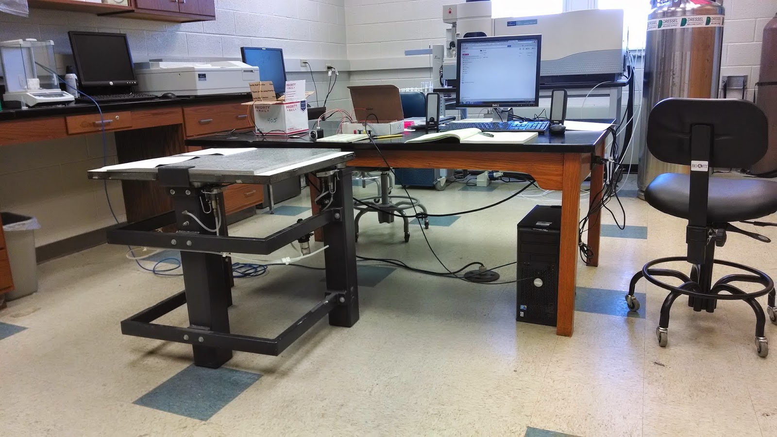
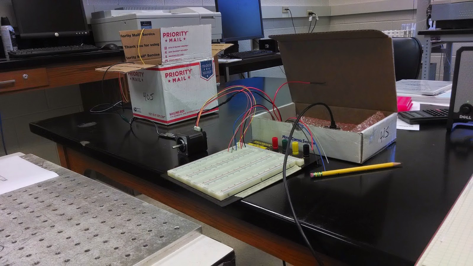
Back to the mechanical side of things, I made a couple of important breakthroughs, but I’m not entirely sure of their implications. I analyzed how the motor control board and our code for the control board works more thoroughly. When I initially ran the code, I found that the setup thought it was at initial coordinate setting of -16,777,216 (units, still need to figure out what the units are). Not remembering what I had left the motor at yesterday, I assumed this might have been just where I left off, although it was highly unlikely. I told the code to move the motor to a position of 0. After this, I proceeded to unplug the motor control board from power and the computer. I closed out all of the code as well. Reconnecting everything, the position remains at 0. I then told the code to move to 100,000 and verify it was at 100,000. Closing and unplugging everything only to reconnect later, I found the position was now 0. I noticed that after a move to 100,000, the motor was at roughly the same position as 0. To verify that 100,000 wasn’t simply a “rotational multiple of 0” (like on the unit circle, 0, 2pi, so forth), I made a move to 50,000, believing that this should be somewhere in half, and give an initialized number. This is not the case however. This will also read 0 on startup, as well as any non-multiple of these. What this means is, the control board does not hold memory after power down. I also noticed that the absolute moves as used in the code, 25,000, 50,000, 100,000, and 700,000 are not multiples of one another, as they do not remain at the same position. What this also means is that there will be a problem with initialization for absolute moves. Any position the motor is in at shutoff will become the new 0 at startup, so absolute moves no longer are absolute. I also have no idea why the code believed the motor was at -16,777,216 at startup.

I found what I thought could be possible Piezo-related subvi’s. All of them are contained within the SimpleMove vi, or within the Piezo-related subvi’s as additional Piezo sub vi’s. This is good, as it means it should be relatively easy to remove the part of the case structure in SimpleMove that contains the code for the Piezo with little repercussions.

Finally, I began exploring the code above SimpleMove. I found that SimpleMove has instances in InitializeLUT, InitTweezers, MoveTrajectory, the main instance of the code, and UseParFile. I began my documentation of MoveTrajectory, although it is quite a complicated bit of code. For tomorrow, I plan to continue to document these vi’s. Also, out of curiosity, I will find what the code believes to be the initial position of the motor.    

BioSAXS Controls Video

Video of System Running: The first computer screen shows a spreadsheet of all the runs with information about each run; what it is, how many seconds its exposed for each image, how many images, and the time that the run began. The second computer screen controls the spec to make each run start and to vary the time of the run. This screen also controls the sample cell to tell it to move the sample left or right, to oscillate and at what step size it should take. The TV screen above both shows what the camera sees so that the oscillations can be regulated and we can be sure that no aggregates or bubbles are in the cell. Above all of this is the sensors for I2, I3, GDoor and the diode. The diode does not give us much information. When I2 and I3 are large, that signifies the strength of the X-rays in the beam.

Week Two: BioSAXS

I accompanied Professor Andresen to the Cornell High Energy Synchrotron Source (CHESS) to run SAXS experiments on various nucleosome arrays. Friday and a large part of Saturday, we modified the experimental setup. We elongated the tubing in the hutch, inserted a beam stop, switched the detector from a 100K pixel to a 200K and began with an X-ray of 200 by 200 micrometers. 

Inside the hutch, overall view of the setup. The long tube farthest to the left was exchanged with the tube on the wall behind to lower the q value. The X-ray beam enters at the far right.
Further to the right the 200K detector can be seen which is the box on the end of the tubing. Right before the detector is a glass plate that the beam stop is placed on. **Fun Fact: Professor Andresen, as a graduate student, painted the maroon square behind the detector.

Then a camera was set up to look at the sample inside the beam mostly to ensure that the sample was centered at the beam and to look for possible air bubbles or aggregates in the sample. At this point the guards and elements of the tube were varied to get the best beam signal throughout the tube with minimal scattering due to the sides of the tubes. Silver behenate was used as a calibration of the beam to find rough values for q to see what range we were working with. All of this was changed in the hopes of lowing the q value, which is the momentum transfer or scattering vector, to a low of 0.004. After the physical setup was chosen and implemented, all the different elements had to be synced with the computer outside the hutch (the hutch is the room where the X-rays are present during experiments).This was what took the most time because so many variables were changed since the last time the G1 hutch was operating. 

Operating system outside of hutch including the real time values of I3 and I2 which give an idea of the strength of the X-rays inside the hutch, the camera monitor that is looking at the sample, and all of the programs that control the beam, guards, sample etc. 
In the image above, Professor Andresen was closing the hutch door and turning the key. This is where the key is placed and the X-rays are turned on. After searching the hutch (pressing two buttons on either side of the hutch and ensuring no one is inside) the door is shut, key is taken and placed in the Station G1 control and the black buttons are pressed on the top right corner of the control box. 

 The element that gave the most trouble was the beam stop which was not in the correct place for running initally and also had different components that continually got in the way of the X-ray beam. This caused the I3 signal to be very low (~16) until it was fixed and showed a signal of ~200. After many hours of centering the beam and correcting the scattering from the sides, we began taking data from our samples. 
We began with the Trimer A which is three nucleosomes together because it is the smallest set of nucleosomes we will look at this weekend. First, distilled water is sent through the sample cell (about 3 times), then ethanol is sent through (about 2 times). At this point the sample cell is mostly clean so we turned on the air to dry the area for about 30 seconds minimum. After all that, we inserted a buffer, closed the hutch, and ran the buffer. This gives us a base line to subtract out any systematic problems against the actual samples. 

View of where the sample is inserted. Between the two plates, a small clear sample cell can be seen. This is where the samples, buffers, water and alcohol is placed and also where the air comes out. The camera is on the opposite side of the beam.  

We ran everything for 5 seconds with 20 images with a ten second break and then once more. After the buffer, we cleaned the sample cell with water, alcohol, and air once more and put the sample inside. We repeated the set up of 5 seconds, 20 images twice for the sample. This procedure was followed for all of Trimer A which included three dilutions (1x, 2x, 4x) for buffers of 10, 50, 100 and 200. 
Today, we are running samples of higher nucleosome arrays. Tetramers and dodecamers (4 and 12 nucleosome arrays respectfully) are much larger structures so the set up had to be modified so that the scattering angles could be measured. This is because larger objects give smaller scattering angles and smaller objects give larger scattering angles. We had some issues with a peak coming off in the z direction from the beam but by changing the guards and the beam stop, this was corrected. Because we are working with the other samples, we lower the beam size to 100 micrometers in the z direction which also lower our intensity so we will be taking longer time intervals when we run. 

Week 2: Friday

Today I worked primarily on experimenting with the motor control VI and documenting the SimpleMove vi and its sub vi’s. I also did a little bit of reading on magnetic tweezers. But first, I’d like to share with you the current setup we have for the lab.

We took the floater table from the nuclear lab and moved it into the middle of the room. Also featured is the new computer.

I started the day by messing around with the motor control board, the motor, and the VI that’s supposed to run it. I improved over my messing with it from the other day by managing to successfully make it rotate in the opposite direction today. Although I initially thought that the code written for the control board would be bug free, I discovered later in the day that there would be certain cases in which the code would break. For example, starting from point zero, it is possible to move the motor in the wrong direction into negative absolute points. This could be bad for the MT setup, as it could result in the motor moving when it cannot physically move due to a barrier. I also found that when just launching the VI, the code does not always recognize what is zero for the motor.

The motor setup: A control board straight out of the box (or in it), a motor, and a breadboard. A USB cable leads to the computer. A power supply runs off of the table to the control board.
A picture of the control board that we are using. It is a Trinamic TMCM 6110 motion control board.

I also ran into issues today with the code that calls the move controls for the motor. Yesterday I attempted to see if deleting parts of that code that don’t pertain to the motor control would allow for it to run even though we don’t have the other parts that the parts of the code that I deleted refer to. Unfortunately, today I found that it still will not be able to run, as the unit calibration and timing sub vi’s will not run due to missing files. It’s possible that if this overhead code that calls the motor control code fixes the problems with zeroing I mentioned earlier, but I’m not 100% sure.

Week 2: Thursday

Today I reviewed the new LabVIEW code sent to us. We finally have our new computer up and running in the lab installed with LabVIEW. I managed to make the motor control board operate the motors through the supplier’s LabVIEW code just as Dr. Andresen had. However, I found that the existing MT LabVIEW code could also run the motors. While I was quite pleased with this, I found it to be somewhat buggy, and had no way to make the motor move in the opposite direction, which is disappointing. I believe it to be a problem with some uninitialized values, which might be initialized or transformed in some other VI in the codeset.

For the rest of the day, I began looking at the SimpleMove.vi, the part of the code that basically tells the motor control to move. It also does several other things, however, it’s not functional right now, since there are several pieces of the code missing. With our optics in order and just waiting to be ordered, it is now my job to figure out how to get this section of the code running again, which should take a couple of days.

Week 2 Wednesday

For the most part this week, I’ve been figuring out the optical system and components that we are going to include in the magnetic tweezers setup. It’s been problematic so far, because we’re having difficulty with the parts list from one of Professor Andresen’s friends. Complicating the situation is the fact that they’re in Singapore, so any communication is delayed significantly.

One of the first problems we have is determining how to focus the collimated light coming out of the objective. This light has to be focused in order to be stored on our CCD. We have a choice of either a f=100 or f=180mm lens. However, we’re unsure if (and what would happen) if we include both lenses in the setup at the same time. Secondly, we need to figure out what type of LED we want as our light source. We’re leaning to using Thorlabs as our main supplier for all of our opto-mechanical and optics equipment for ease. So, for the most part of this afternoon, I’ve been chatting with a tech-adviser from Thorlabs for help with selecting the LED and the appropriate opto-mechanical components. Right now we’re leaning towards a red (625nm) LED w/ an output power of 1000mA. To collimate the LED, we’ll be constructing our own collimator out of different Thorlab stuff. We’ll be using an aspherical lens with AR coating in some appropriate housing to collimate the light from the LED. This housing will attach to the LED itself. Of course, the main problem now is making sure that the whole list of everything we need is complete, and get everything ordered.

Week Two: Mike Mike Mike Mike! Guess what day it is!?!

This morning, I reanalyzed the cobalt- only samples on the ICP, exported the raw data, and added the information to the graphs I made yesterday. The fraction of charge neutralized by cobalt was within the standard deviation from the first run but the individual concentrations of cobalt and phosphorus were significantly lower than yesterday. Although the second run had much lower concentrations, the trendline for both ions traced the same as the first run. This afternoon, I have been catching up on my reading about DNA, nucleosomes, SAXS and studies related to my experiment.