Category: Uncategorized

When we first started out our research this summer we were working on finding the best digestion for our chromatin. Digestion, simply put, is a way to get a fragment of a larger substance, in our circumstance, we are digesting chromatin to get nucleosomes. Our Senior Investigative Researcher (SIR) Macyn Rosay helped us to begin this process and slowly got us to do the process on our own. For the past week, we have been doing the digestion independently, looking for the best time for the 15-unit digestion. In the prior week, we had done a unit digestion that led us to 15 units the best for the digestion of our chromatin (so many gels). Unit digestion is how to find the baseline of Micrococcal Nuclease (MCN) to get the most amount of nucleosomes. From there we did a time digestion that ranged from 10 minutes to 55 minutes, and from this digestion, we concluded 30 minutes was the best for nucleosomes (see Fig. 1). Since 30 minutes was our blessed digestion we had (finally) moved to the next step which is mass digestion (only one more gel yay). The digestion process will be explained more in-depth later, for now, enjoy our fluorescent gel.

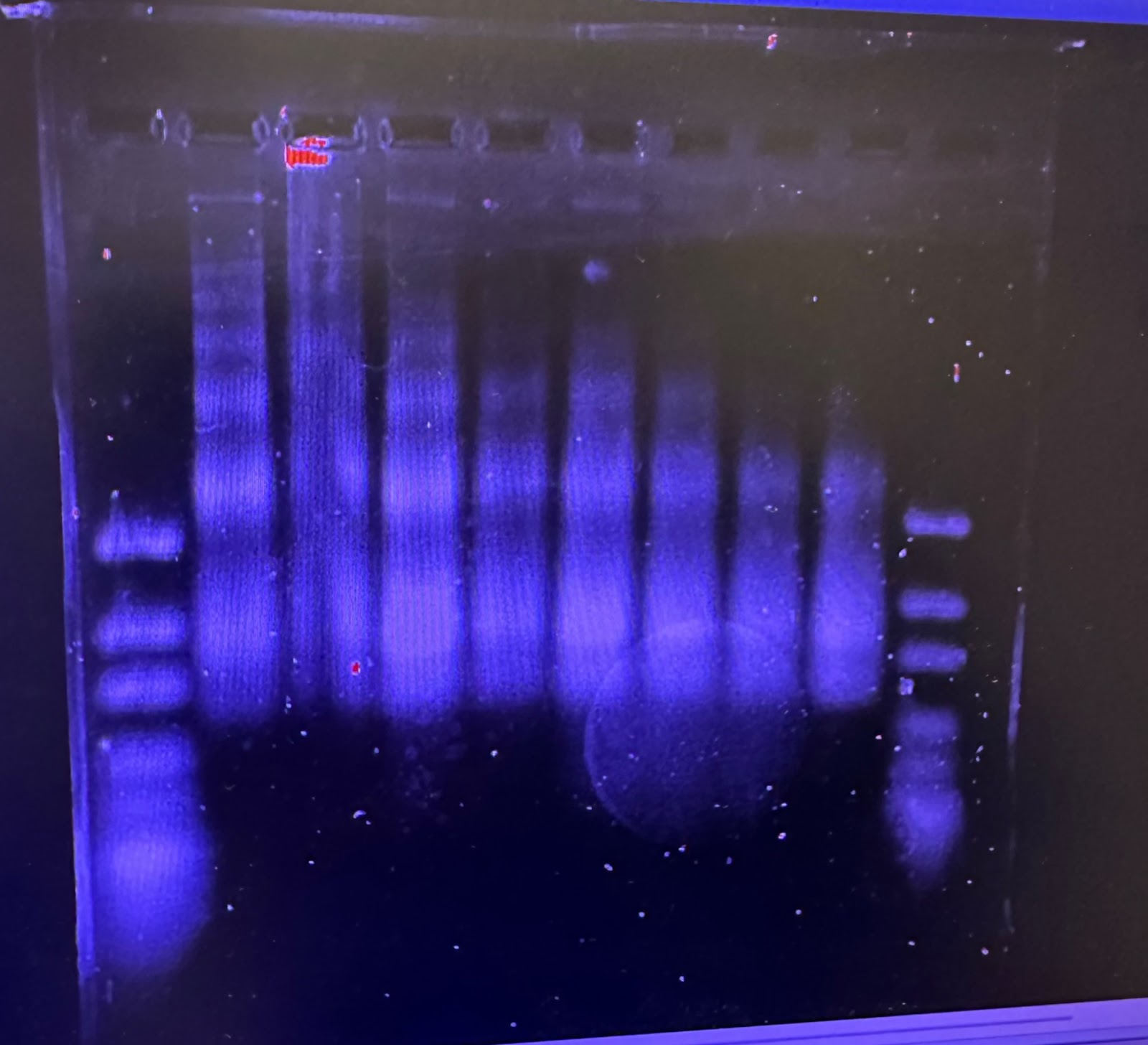
Figure 1: 15 unit Time Digestion of Chromatin

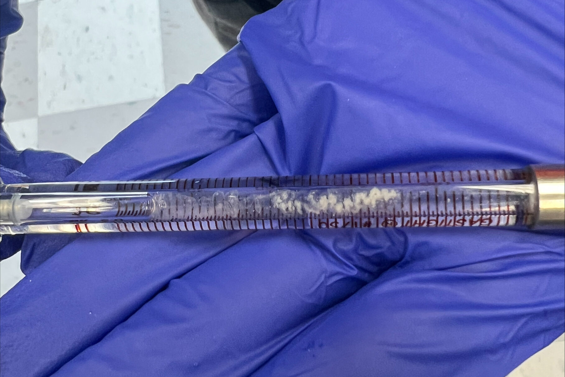
Once we (finally) made a good gel, we could move on. We spent the rest of the day digesting chromatin. We had a sample of 50 mL of chromatin that we separated into two separate test tubes with 25 mL in each just to make sure if we mess up (which we won’t), we are not using up all of the chromatin that we already have. If we do, then its back to the farm to get more chicken blood! 

We then added 4.5 mL of MCN to each of the two test tubes filled with chromatin and then centrifuged them. After that, we equally separated this new solution (chromatin + MCN) into 5 test tubes with 5 mL each and heated these samples for 30 minutes at 37 ℃. It was now time to make (another!) gel (and listen to Lana Del Rey of course).  Once 30 minutes had passed, we combined the 5 samples and added 1.25 mL of EDTA before putting it on ice for about 10 minutes (time for more Lana). 

Next, we prepared two samples for the gel, one with 5 μL of chromatin, 5 μL proteinase K, and 0.5 μL SDS. The other sample had 5 μL of digested chromatin rather than the undigested chromatin. We then placed these two samples into the isotemp for 50 minutes at 50 ℃. 

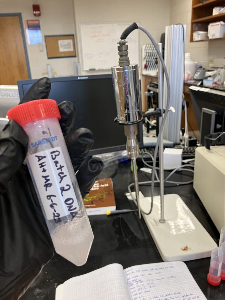
It was now time to move on to a higher-power centrifuge, which Professor Andresen taught us how to use. We added the digested chromatin to two centrifugal filter units and let those spin for about 10 minutes. In the meantime, we made a sample of 1.0 M NaCl which we later used to make 1.0 L of TEM buffer (Tris, EDTA, NaCl). 

We then finished the digestion and loaded the gel before letting it run for about 2.5 hours. While it ran we took a lunch break at the world-renowned Bullet Hole (it is THAT good). Once they were ready, we analyzed the gels and got the thumbs up from Professor Andresen (YAY).

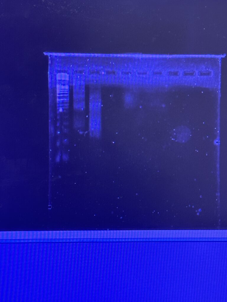
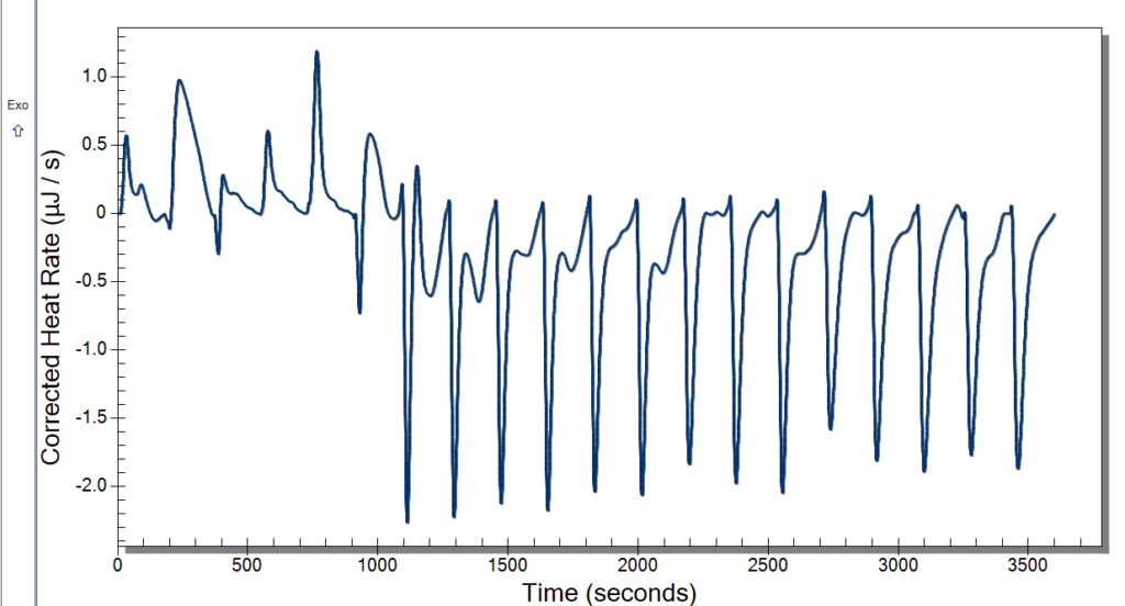
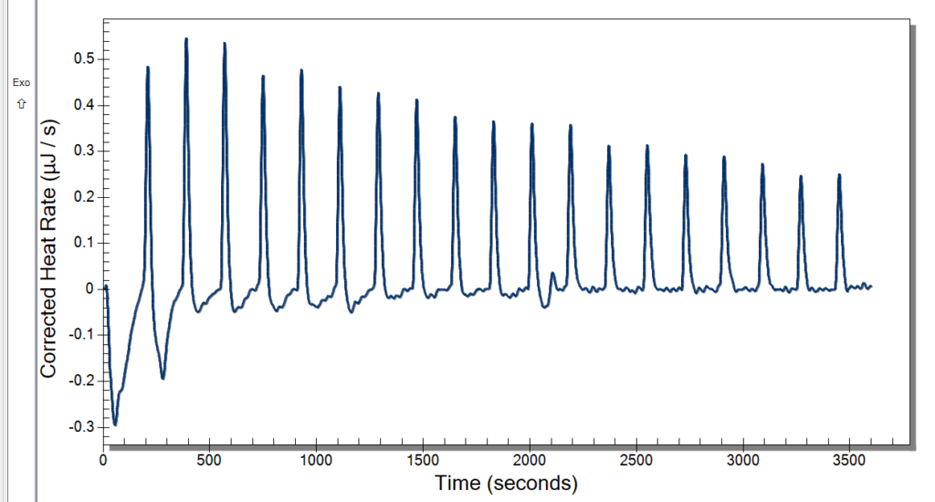
Figure 2: Digestion of Original Chromatin & 30 min Digested Chromatin

So through some rough patches in the first few weeks, we made a breakthrough, but even when we were going insane we always had great music playing.

Signing Off
JIM 2 (Eden) and JIM 3 (Kyle)

The goal of the first week was to become familiar with GROMACS, the program used to computationally simulate processes of nucleic acids, and successfully simulate research with familiar results. After general tutorials and practices, I recreated part of the experiment done by Jejoong Yoo and Aleksei Aksimentiev in 2012 (“Competitive Binding of Cations to Duplex DNA Revealed through Molecular Dynamics Simulations”), where they added +1, +2, and -1 ions (Na, Mg, and Cl) to DNA in a box of water. The goal of these simulations is to first find the bulk concentration (the base number of ions surrounding the DNA) of each ion, and then the bound concentration. The bound concentration is found using radial integration of sections surrounding the DNA, and tells us how many ions cluster around the DNA.

In Figure 1, we can see the bulk concentration where the concentration levels out around 25 A. The bound concentration is the area under the peaks. The graphs visualize the gathering of ions around the edge of the DNA. In this example, we can see that when there are equal amounts of Mg and Na, there is a significantly larger amount of magnesium clustered around the edge of the DNA. However, the next part of the experiment that I emulated was increasing the amount of sodium a significant more amount than the magnesium, which produced different results.

Analyzing the graphs and the data points of Figures 2 and 3, we find that sodium and magnesium/chlorine have an inversely proportional relationship; as we increase the sodium concentration, the magnesium and chlorine charge decreases. This shows the “competition” aspect; when sodium increases, it pushes other ions away from the DNA. Comparing the figures, we can see that our simulation data matches the study’s results, which shows that we completed the simulations correctly and can trust our results. Now that we know how to simulate these processes accurately, we can move on to unfamiliar research.

Hi everyone! I’m Aubrie, a rising sophomore physics major here at Gettysburg College. I’m excited to be working in Professor Andresen’s lab this summer for X-SIG and to work with my wonderful colleagues Macyn, Sofia, and Aston. My research is in collaboration with Macyn here at the beginning, and we will be researching the The Entropy and Enthalpy of DNA systems continuing from Tam’s work last summer. This past week we haven’t exactly started our individual projects yet, but we have started learning about the equipment available to us and how we might use it in conjunction with our research.

We started the week by learning proper pipette technique and practicing seeing our accuracy. It took some time, but I eventually was able to get the hang of it. I really struggled with the pacing of releasing the button, so I kept getting air bubbles in the tip which caused me to be under the expected amount. We also made salt stocks using NaCl and Cobalt Hexammine.

Tuesday involved us replicating an experiment that observed how DNA aggregates with Cobalt Hexammine. We learned how to make our DNA samples, put them through the centrifuge, and measured the concentration using the Nanodrop. We then added 20 microliters of Cobalt Hexammine and repeated those steps to see how DNA falls out of solution. We took a break in the middle to go for lunch at Food 101, but it was closed for renovations, so we ended up at Montezuma. I got the fajita burrito, and it was delicious.

We started Wednesday morning by making some DNA samples to use in the Circular Dichroism (CD) in the Science Center. We took an adventure to Prof. Buettner’s lab and got training on the CD, and later we ran our samples on the CD ourselves. I learned more about coding as well, and I feel a lot better about it already.

Thursday started out a bit rough. We were cleaning and ran out of water. A seemingly boring trip to get water ended up with a broken water jug and having to clean water off the floor. We were luckily able to borrow one from Prof. Thompson. Then we trained on the ICP with Prof. Andresen and that afternoon we trained on the ITC with Prof. Thompson. There is a lot to it, and we plan to replicate an experiment with it this week to see if we can get accurate results.

Friday was calm. I spent the morning reading a thesis from a former student and a paper that relates to it. I took some notes and googled a lot of terms. That afternoon we had personal meetings with Prof. Andresen to discuss how everything was going.

Monday has been pretty good. We started the morning with our group meeting, and I had some code issues, but it was a pretty easy fix. We discussed the best ways to read scientific papers as well. Macyn and I started a replication experiment with the ITC. Our first results were pretty rough, so we stopped the machine because we clearly made mistakes. Our second results were really good, and our third results were not consistent. We cleaned up after that one.

If you remember from my last blog post, we were about to embark on a new journey. After collecting a lot of data on zinc and what it does to DNA, we want to see if this change is reversible or not. Does the zinc bind so tightly that it cannot be washed away? Answering this question is what I’ve been up to this week. In order to do this, we took some samples of DNA in a 300mM zinc solution, and tried to get all the zinc out via centrifuge. We put the samples through a special filter that lets everything but DNA pass through, and then we add NaCl, MgCl2, and Tris buffer five times, running them through the centrifuge each time. After this was all done, I ran the samples through the CD spectroscopy machine, so we could see any changes in the DNA structure.

This is our latest graph, and we can see that DNA that has been washed with salts and a buffer looks very different from DNA in zinc solution that has not been washed. We can interpret this as the zinc unbinding from the DNA, which makes the peak at 275 nm revert back to how it was before zinc was added. However, we can still see some differences between the washed and unwashed DNA. The through at 245 nm is greater for the washed solutions, but is very similar for the DNA in plain water, and the DNA in zinc.

I am currently in the process of redoing this whole experiment. I hope that the new graphs will corroborate the data that I have already acquired, and help me analyze more accurately the differences between washed and unwashed DNA. Until then, I do think that we have some promising data, and I look forward to elaborate more on this experiment.

What have we been up to? For starters, the project about measuring Zn2+ binding to DNA has really taken off. We started by doing some samples of DNA in NaCl and MgCl2, which you might remember from our previous blog post. We did those several times to try to get some results that showed a change in the DNA structure. We ran all of our samples in the CD spectroscopy instrument, which measures how long it takes for DNA to unwrap. This time, we measured over the right span (320 nm to 200 nm), which means we can now read our data!

 What we wanted from these graphs was to observe a difference in the magnitude of the peak and trough of the graph, which was proportional to the sodium and magnesium concentration. In these graphs, it is possible to see that the concentration of the sodium and magnesium is directly proportional to the change in the DNA, however, we do have some outliers. Nonetheless, we decided we were ready to move on to the next step of the project, measuring the effects of zinc binding to DNA. We made two sets of similar Zinc and Magnesium samples, with varying concentrations, with the hopes of getting similar (but better) results to the ones above. We are doing both zinc and magnesium samples in order to compare the changes, to see if it’s the +2 charged ions that is causing the change, or the zinc itself. Then, we will do it all over again until we have a significant batch of good data.

We will also be looking to see if this change is reversible, or if the zinc binds so tightly to the DNA that it cannot be washed away. This will be achieved by exposing the DNA to zinc and later washing it with Tris, NaCl, and MgCl2.

Here are our latest results, which look very promising! We also learned a very handy tool to make our graphs look better and more accurate. By normalizing the line of each sample with the experimentally measured concentration of the sample, we are able to get rid of any variation read by the CD that comes with human error when making the samples.

Hello everyone! Andresen Lab Crew Summer 2022 here! We are here to give you guys a rundown of our first  week of research. For starters, we are working with DNA (I know right!!). Aisha and Sofia will be collaborating on the same projects; Measuring the Kinetics of the Disassembly of Mononucleosomes and Measuring Zn²⁺ binding to DNA, while Tam will be independently working on The Entropy and Enthalpy of DNA systems.

The Golden Trio at Golden Hour

On our first day, we learned the basic skill of pipetting. We pipetted water in order to get a grip on the basics of pipetting before proceeding to pipette different solutions and liquids. Professor Andresen wanted us to use each pipette to measure the same amount three times, with the hopes of eventually getting a percent error below 5%.

On Tuesday we started the day by making DNA stock, which we would be using in all of our samples. We started out by measuring 0.08 grams of DNA. We put the DNA aside and pipetted (with our recently mastered pipetting skills) 7840 microliters of water into a 50mL tube. We then pipetted 80 microliters of TRIS solution and 20 microliters of EDTA solution into the tube, in order to make a TE buffer. We put the DNA in the tube and mixed it in the vortex mixer for a while, in order to break up most of the DNA. After that, to make sure the DNA was really broken up, we put it in the sonicator for several rounds. Now we had a 8mL sample of 10mg/mL of DNA, which we then diluted into a 1mg/mL sample so its concentration could be double checked in our spectrophotometer. After several rounds of checking the concentration, we got around 0.8 mg/mL, which is considerably less than what we theoretically had. However, the next morning we repeated the process and measured our concentration to be around 1mg/mL, so success!

On Wednesday, we started by mixing our DNA stock with NaCl and MgCl₂ solutions. Our goal was to make 5mg/mL of DNA in different concentrations of NaCl and MgCl₂. We used the formula M₁V₁= M₂V₂ (which looks the same as the momentum conservation formula) to find the amount of NaCl and MgCl₂ we needed to get the right concentration for our solutions. After that, we had to dilute all of our samples by a factor of 5 because that was the concentration that our spectrophotometer can measure. Most of our results were within a reasonable range (the expected values of DNA’s concentration was 1000 ng/microLiter).

Today (Thursday), we spent the day in our collaborator, Dr, Buettner’s lab, using the CD machine to measure how long it’ll take for the DNA to unwrap, (the nucleic acid inside the DNA). After measuring all 11 of our samples, professor Andresen gave us a coding crash course, so we could start interpreting and graphing our results using Jupyter. However, we realized that we measured our DNA samples within a range that was too narrow, so we have to go back tomorrow and do it all over again. Nonetheless, we will not be taken aback by a small setback, we will come back stronger than ever tomorrow! 

The Andresen Lab is back in full swing again! We’ve got a new crew that is ready to do some great science. You should soon be hearing from Aisha, Sofia, and Tam about all of the great work they are doing and plan to do.

If you really want to make sure you don’t miss anything, you can subscribe to our RSS feed. Also, feel free to check out our (static) Andresen Lab web page to find out more about the lab.

Hello again. It’s Matt back with some progress updates on my research. For starters, I got it working!

As a reminder, the purpose of doing this is to simulate a single strand of DNA, the one in the middle, as if it were in vitro. Since we can’t simulate the entirety of a strand of DNA (it’s far too large), we take a small portion of it and hope that the insights we glean can be applied, or at least give us some insight into the whole DNA strand. There is also a slight change that you may have picked up on: the DNA has been rotated around the y-axis. This is purely for our sake in doing the analysis; it’s challenging as-is to work with 4D data sets (after we run the DNA simulation through the online web server that does all the math for us we get back data that when we plug it into matplotlib we get a 4D data set: the x, y, and z coordinates as well as the electric potential at all points), adding in another level of complexity in having to consider the x-axis as the z-axis, for instance, just adds needless confusion. It took me about two days to implement this rotation as the way I attempted first was to essentially make another function in my program that rotates the coordinates of the original DNA strand before I copy it everywhere. Unfortunately, rotations in 3D are hard and I couldn’t get it working. Luckily, I found something online that simplified the work a ton: the program we’ve been using to visualize the DNA (where the picture came from), VMD, actually allows you to change the locations of the DNA and spit them back into the original file. With 6 lines of code, the DNA strand was rotated and I could use my original program with no edits.

Now, our goal is analysis. I mentioned above that we will be using matplotlib, a graphing package for Python, in order to accomplish this. Basically, what we want to do now, is take the big long sheet of electric potentials that we have at every point in the simulation and trim it down to only the data we care about: the data inside a smaller-than-the-small-hexagon (i.e. inside a 28nm radius hexagon centered around the central DNA strand). Again, our goal is to simulate this singular DNA strand; the rest of the data isn’t representative of this goal and can be ignored for our analysis, the only reason it exists in the first place is because the potential at a given point depends on the potential at all the points around it. Once the data we want is selected (which is probably the hardest part of the rest of the project, 3D plots in matplotlib are no joke) we can then do some math on our end to figure out the excess number of ions that are present around the DNA strand according to the Poisson-Boltzmann equation. If you remember from the last post, this is the entire point of the project! If we can get the number of these ions we can begin work on publishing the paper and the sweet sweet publishing credit can be added to my resume! One step at a time, but every step forward is one step closer to grad school.