Author: Prof. Andresen

After successful preparation of calibration standards yesterday, I made 86 samples (below) to run through the ICP-AES next week. Next week I will also be preparing more calibration standards and samples.

Today, we ran our calibration samples in the ICP-AES to get an idea of how precisely we made our samples and to learn how to use the machine. After we finished running the samples and analyzing the results, I visited Professor Thompson’s lab in the Chemistry department where he outlined the process we will follow for the next couple weeks. Today, I diluted a solution of spherical gold nanoparticles he prepared, and treated them with polystyrene sulfonate and sodium chloride. This mixture needs to sit over night so the polystyrene sulfonate has time to absorb onto the nanoparticles surface. Tomorrow, I will centrifuge down the treated nanoparticles and begin characterizing both the treated and untreated samples.

Looking forward to an interesting and exciting summer! These past few days I have been organizing and gathering background information by reading scientific papers so I can begin research soon. Today we ran standard samples through the ICP-AES to learn how the machine works as well as determine the precision of our standards. Hopefully later this week I will be able to run some samples through the ICP-AES and begin to look at ion binding competition in DNA-arrays!

Today was the first day of summer research! Ambitious plans were laid, literature was read, and calculations were made. My project will focus on the interactions between gold nanoparticles and DNA. My goal for the next couple weeks will be to synthesize polyelectrolyte coated gold nanospheres and characterize their features. Then I will run equilibrium dialysis and atomic emission spectroscopy (ICP-AES) on these nanospheres with different concentrations of ions. I’m looking forward to an exciting summer!

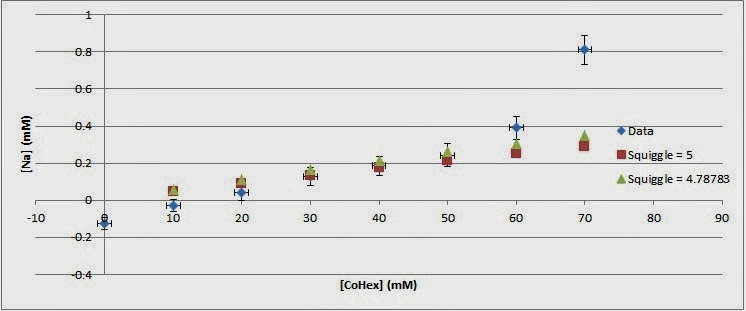
I averaged all of the ICP runs from the past two weeks and compiled them onto one Excel spreadsheet. I then began looking at the Na/Co ion competition more thoroughly using the article Prof. Andresen and John Giannini collaborated on a few summers ago, “Ion Competition in Condensed DNA Arrays in the Attractive Regime” as a guide. I tried to use the ion binding model used in the article to analyze the relationship between the number of ions near the DNA arrays and the solution’s ion concentrations. This involved finding a constant, ξ, to relate the two sets of numbers (aka. the squiggle). After rearranging the formula given for a simplified ion binding model, I found a ξ for each data point. I took a rough average and an actual average and compared the values found using the ξ against the data from the ICP (shown below).

I haven’t been blogging lately because I broke the USB wifi adapter on the computer I’ve been working on. I accidentally stepped on it. So, here’s a run down of everything I’ve been doing lately, with pictures. Also, the magnetic tweezers are almost finished, minus a working flow cell.

As of today, this is what the Tweezers look like:

This is the light source. It is a red Thorlabs LED with a wavelength of 625nm. The LED has been collimated by an aspheric condenser lens, f=20mm. In MT, it is important to have a collimated light source with a low coherence length, as this allows for a better generation of diffraction rings around the beads, which is essential in taking measurements. The long, ventilated part on top of the LED is the heat sink. The LED is being held by a kinematic mount attached to our rail system. This allows for greater control over the positioning of the LED and direction of the light source.

Directly under the light source are two motors and the magnet setup. Here you see the rotary motor, which has been coupled to a sled moved by a stepper motor, which in turn has been mounted on the rails. The rotary motor holds the magnet holder, and allows for rotation of the magnets. By rotating the magnets, we can apply a torque to the magnetic beads, and thus, the DNA (or whatever is attached to the bead). The stepper motor that controls the sled allows for moving the rotary motor up and down in space, and therefore controls the strength of the force being applied to the beads (magnet closer to the bead, stronger force).

This is the magnet holder, and attached to the magnet holder are the magnets. They are two Neodymium magnets.

Here we can see the full-middle setup of the MT. Underneath the rotary motor is the XY table. We will couple our flow cell (still in production) to the top of this. The XY table allows manual movement of the flow cell in X and Y directions (i.e. horizontal to this picture.

This is the view underneath the XY stage. Not shown here is the microscope objective, which is a Nikon 100X oil-immersion objective. The objective attaches to the objective holder, which has been coupled to another sled controlled by a stepper motor. This stepper motor allows for control of the focus of the magnified image of the sample cell. By moving the objective closer or further away from the sample, we can change the focus of the image.

Light exiting the objective is reflected by this 45 degree mirror. I have momentarily removed it from the MT setup in order to make access to the underside of the MT easier. The mirror reflects the light to the camera setup.

And this is the camera setup. It consists of a lens tube, a 100mm aspheric focusing lens, and a JAI-Pulnix CCD camera. The light collected in the tube is focused onto the CCD, which then transmits black and white images of the sample to the computer.

This is the entirety of the MT setup. So, how does it work, and what is it’s purpose? You’ll just have to wait for another blog post…

Today, I tried to normalize the cobalt-only data several ways. I’m still not sure if I did it right or if WinLab did it correctly on the computer. Both ways I normalized it lead to larger error bars (not by much but still). Overall they all look pretty much the same. Because of this, I made a PowerPoint of my overall results for this set of data off of the original data instead of the reprocessed. A few days ago I thought my error bars were great overall, then today I realized I forgot to multiply one set by three so now they are not that good. Hopefully they are good enough when I add a few more runs of samples onto it in the next three days that have the extra buffer.

All three of the ways I tried to look at my data. All pretty much the same except for slightly different error bars.

This morning I created new calibrations that included 0- 2.5 ppm Na to see if there are any effects due to sodium in the cobalt- only samples. I then diluted another set of sample solutions to run. This afternoon, I attempted to run the samples with the new calibration solutions but the sodium was very very off. I used a new stock solution of Na to make the solutions so tomorrow I am going to use the old and see if that fixes the problem. If not, I might have to scrap the new calibrations and simply use the old without sodium. The rest of the afternoon, the physics department tie dyed behind the science center.

This morning, I ran the remaining samples from the other dilution of the cobalt- only series. They had concentrations similar to the runs I have made this week so I must have made a mistake a month ago when I ran them. This afternoon, I made more samples to run and ran a combination of all the samples I have made this past week. The last run had an overall trend of lower concentrations for Co, P and the internal standard Sr. Hopefully I can use the standard to correct for this tomorrow.

Steve and Prof. Andresen are super excited about making the motors move!! (and other stuff probably but I wasn’t paying attention)

I recreated a 30x dilution set of the cobalt-only samples and got the same result as yesterday. Although the ion concentrations are about a factor of 10 lower than the previous data, the charge ratio of cobalt for both dilutions are within each other’s uncertainties. Tomorrow I’m going to play with the old samples to see if the factor of 10 still exists in the samples and then possible make new samples of that dilution and run it to compare to the old results.